Create LTSpice Custom Plot
LTSpice is a largely used simulation tool for electronics. However, when required to export the plots generated by the simulations, it lacks some customisation and configuration flexibility.
Either the MacOs or Windows version of the software have the tools add text, lines, rectangles and circles to the Plot. As well, a Plot Configuration file (*.plt), which holds all plot display configuration can be saved for reuse.
Editing the plot configuration file give the possibility to create plots with a nice visual appearance and annotate them with complex information.
To be able to edit the plot configuration file first some understand of how LTSpice save information to the plot configuration file is required.
Various customisations can be done on the Plot Configuration file that are not described on this article. However, it can give a very good starting point.
Colour Numbers
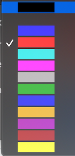
Each colour on the LTSpice environment has a number associated to it, from 1 to 13.
The picture below shown the main colours available on LTSpice [1..13].

Example:
| Colour | Number |
|---|---|
| Black | 1 |
| Blue | 3 |
| Red | 4 |
| … | … |
Line Types
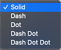
As colours, LTSpice uses numbers to identify the line type as below.

| Line Type | Value |
|---|---|
| Solid | 0 |
| Dash | 1 |
| Dot | 2 |
| Dash Dot | 3 |
| Dash Dot Dot | 4 |
Text Alignment
Text alignment value is a combination of alignment type value and colour number.
| Alignment | Value + Colour |
|---|---|
| Left: | 256 + Color # |
| Right: | 512 + Color # |
| Center: | 4096 + Color # |
| Top: | 1024 + Color # |
| Bottom: | 2048 + Color # |
Example: Blue text on Left: 256 + 3 = 259
Plot configuration file elements
1. Lines
Lines are defined by the syntax below:
1
Line: "<ASSOCIATED VERTICAL UNIT>" <COLOUR #> <LINE TYPE #> (<X Start>,<Y Start>) (<X End>, <Y END>)
Example:
1
Line: "dB" 4 0 (9000,316227.766016838) (50000,316227.766016838)
On the example above the vertical unit is in dB, Colour is red, Line type is Solid, X start/end is in Hertz and the Y start/End is defined as 10^(value_db/20).
The same Line syntax is applied for Rectangles, Circles and Arrows. Just Replace “Line: “ by “Rectangle: “, “Circle: “ or “Arrow: “
2. Text
To add text to the plot via Plot configuration file use the following syntax:
1
Text: “<VERTICAL UNIT>” <TEXT ALIGN + COLOR> (<X>, <Y>); <TEXT>
Example:
1
Text: "dB" 515 (3000000,316227.766016838); DIFFERENTIAL MODE
On the example above the vertical unit is in dB, Text in blue right aligned, X is in Hertz and the Y is defined as 10^(value_db/20).
3. GridStyle
Syntax:
1
GridStyle <NUMBER>
| Number | Status |
|---|---|
| 0 | grid off |
| 1 | grig on |
Examples
Below are some examples of Plot Configuration File (*.plt) edited.
Ex. 1 - EMC Test
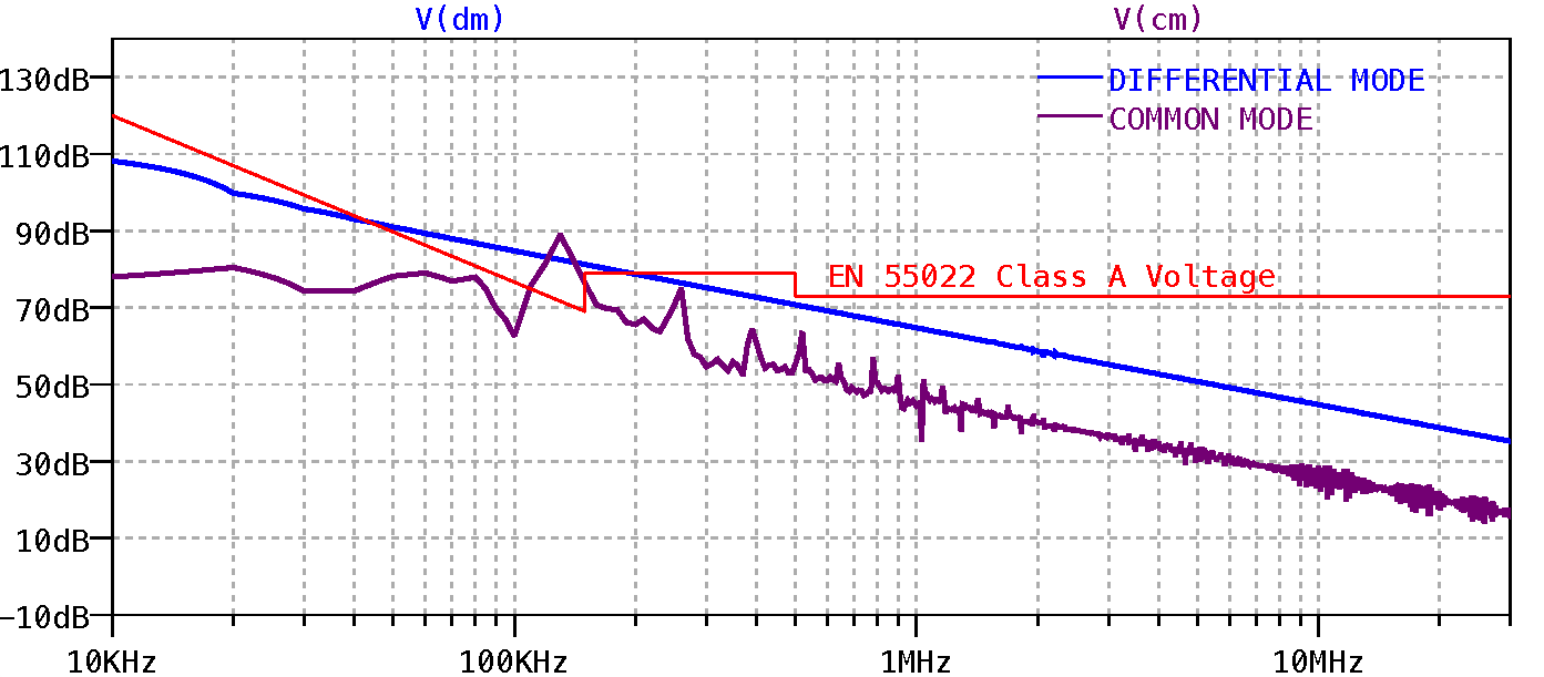
On this example the Plot Configuration file is edited to show the EMC limit line and add annotation text to the plot.
1
2
3
4
5
6
7
8
9
10
11
12
13
14
15
16
17
18
19
20
21
22
23
[FFT of time domain data]
{
   Npanes: 1
   {
      traces: 2 {524291,0,"V(dm)"} {524299,0,"V(cm)"}
      X: ('M',0,10000,0,3e+07)
      Y[0]: (' ',0,0.316227766016838,10,1e+07)
      Y[1]: ('_',0,0,0,0)
      Log: 1 2 0
      GridStyle: 1
      PltMag: 1
      Line: "dB" 4 0 (10000,1000000) (150000,2818.38293126446)
      Line: "dB" 4 0 (150000,2818.38293126446) (150000,8912.50938133747)
      Line: "dB" 4 0 (150000,8912.50938133747) (500000,8912.50938133747)
      Line: "dB" 4 0 (500000,8912.50938133747) (500000,4466.83592150963)
      Line: "dB" 4 0 (500000,4466.83592150963) (30000000,4466.83592150963)
      Line: "dB" 3 0 (2000000,3162277.66016839) (2900000,3162277.66016839)
      Line: "dB" 11 0 (2000000,1000000) (2900000,1000000)
      Text: "dB" 260 (600000,8912.50938133747) ;EN 55022 Class A Voltage
      Text: "dB" 259 (3000000,3162277.66016839) ;DIFFERENTIAL MODE
      Text: "dB" 267 (3000000,1000000) ;COMMON MODE
   }
}
This configuration file generate the following plot

The LTSpice simulation files for this example can be downloaded Here
Ex. 2 - Low Pass Filter
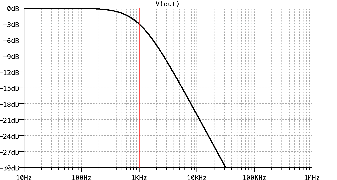
On this example the Plot Configuration file is edited to show the -3dB and Cut frequency lines of a Low Pass filter.
1
2
3
4
5
6
7
8
9
10
11
12
13
14
15
16
[AC Analysis]
{
   Npanes: 1
   {
      traces: 1 {524290,0,"V(out)"}
      X: ('M',0,10,0,1e+06)
      Y[0]: (' ',0,0.0316227766016838,3,1)
      Y[1]: (' ',0,-90,9,-0)
      Log: 1 2 0
      GridStyle: 1
      PltMag: 1
      NeyeDiagPeriods: 0
      Line: "dB" 4 0 (10,0.707945784) (1000000,0.707945784)
      Line: "dB" 4 0 (1000,0) (1000,1)
   }
}
This configuration file generate the following plot

The LTSpice simulation files for this example can be downloaded Here
Tools
A spreadsheet to help to calculate the Line: and Text: coordinates can be download here.
Conclusion
LTSpice is an excellent tool that can be improved with simple tricks. Know how the software uses the Plot Configuration give the possibility to create very complex and visual appealing plots.